LSTM Single Variate Implementation Approach: Forecasting

Learn more about time series forecasting, a crucial analytical technique that helps businesses and researchers predict future trends based on historical data.

Rajat Toshniwal

May. 07, 24 · Tutorial

Like (1)

Save

496 Views

Time Series Forecasting: Single Variate

In today's data-driven landscape, businesses across industries are continually seeking ways to gain a competitive edge. One of the most powerful tools at their disposal is time series forecasting, a technique that allows organizations to predict future trends based on historical data. From finance to healthcare, time series forecasting is transforming how companies strategize and make decisions.

What Is Time Series Forecasting?

Time series forecasting involves analyzing data points collected or recorded at specific time intervals. Unlike static data, time series data is chronological, often exhibiting patterns like trends and seasonality. Forecasting methods leverage these patterns to predict future values, providing insights that are invaluable for planning and strategy.

Some Use Cases of Time Series Forecasting

Sales Forecasting

Retail businesses use time series forecasting to predict future sales. By analyzing past sales data, they can anticipate demand, optimize inventory, and plan marketing campaigns.

Stock Market Analysis

Financial analysts employ time series forecasting to predict stock prices and market trends. This helps investors make informed decisions about buying or selling assets.

Weather Prediction

Meteorologists use time series forecasting to predict weather patterns. This data is crucial for agriculture, disaster preparedness, and daily planning.

Healthcare Resource Planning

Hospitals and clinics use forecasting to anticipate patient influx. This helps in managing resources such as staff, beds, and medical supplies.

Energy Consumption Forecasting

Utility companies leverage time series forecasting to predict energy demand. This enables efficient management of power grids and resource allocation.

Forecasting Techniques

Forecasting techniques include:

Statistical Analysis
Machine Learning Algos like ARIMA
Neural Networking (RNN): LSTM

LSTM

LSTM networks are specialized neural networks that handle sequences of data. Unlike regular feedforward neural networks, LSTMs have loops that allow information to persist, making them ideal for tasks where context over time is crucial. Each LSTM cell consists of three parts: an input gate, a forget gate, and an output gate, which regulate the flow of information, allowing the network to selectively retain or forget information over time.

More details can be found in the video "Long Short-Term Memory (LSTM), Clearly Explained."

In this tutorial, we are going to focus on the single variate LSTM analysis. Soon I will be publishing an implementation approach for multivariate analysis.

Main Code

Importing Libraries

      Python
     
 

     import tensorflow as tf
import os
import pandas as pd
import numpy as np
import matplotlib.pyplot as plt
from sklearn.preprocessing import MinMaxScaler
from keras.preprocessing.sequence import TimeseriesGenerator as TSG
from keras.models import Sequential
from keras.layers import Dense
from keras.layers import LSTM
from tensorflow.keras.models import load_model
from tensorflow.keras.callbacks import ModelCheckpoint
import  tensorflow.keras.optimizers as optimizers
import seaborn as sns
import statsmodels.api as sm
    

Loading the data from the CSV file, this is beverage sales data. Then column update changes Unnamed: 0 to date. Convert the entries in the date column from strings (or any other format they might be in) to datetime objects. The range function generates a sequence of numbers starting from 1 and ending at the total number of entries in the DataFrame (inclusive). This sequence is then assigned to a new column called sequence.

      Python
     
     import pandas as pd

# Load data from a CSV file into a DataFrame
dfc = pd.read_csv('sales_beverages.csv')

# Rename the column from 'Unnamed: 0' to 'date'
dfc = dfc.rename(columns={"Unnamed: 0": "date"})

# Convert the 'date' column from a string type to a datetime type to facilitate date manipulation
dfc["date"] = pd.to_datetime(dfc["date"])

# Add a new column called 'sequence' which is a sequence of integers from 1 to the number of rows in the DataFrame
# This sequence helps in identifying the row number or providing a simple ordinal index
dfc["sequence"] = range(1, len(dfc) + 1)

# Display the modified DataFrame
dfc

	DATE	Sales_Beverages	Sequence
0	2016-01-02	250510.0	1
1	2016-01-03	299177.0	2
2	2016-01-04	217525.0	3
3	2016-01-05	187069.0	4
4	2016-01-06	170360.0	5
...	...	...	...
586	2017-08-11	189111.0	587
587	2017-08-12	182318.0	588
588	2017-08-13	202354.0	589
589	2017-08-14	174832.0	590
590	2017-08-15	170773.0	591

591 rows × 3 columns

Exploring the Data

      Python
     
     print('Number of Samples = {}'.format(dfc.shape[0]))

print('Training X Shape = {}'.format(dfc.shape))

print('Index of data set:\n', dfc.columns)

print(dfc.info())

print('\nMissing values of data set:\n', dfc.isnull().sum())

print('\nNull values of data set:\n', dfc.isna().sum())

# Generate a complete range of dates from the min to max
all_dates = pd.date_range(start=dfc['date'].min(), end=dfc['date'].max(), freq='D')

# Find missing dates by checking which dates in 'all_dates' are not in 'df['date']'
missing_dates = all_dates.difference(dfc['date'])

# Display the missing dates
print("Missing dates are ", missing_dates)

Number of Samples = 591
Training X Shape = (591, 3)
Index of data set:
 Index(['date', 'sales_BEVERAGES', 'sequence'], dtype='object')
<class 'pandas.core.frame.DataFrame'>
RangeIndex: 591 entries, 0 to 590
Data columns (total 3 columns):
 #   Column           Non-Null Count  Dtype         
---  ------           --------------  -----         
 0   date             591 non-null    datetime64[ns]
 1   sales_BEVERAGES  591 non-null    float64       
 2   sequence         591 non-null    int64         
dtypes: datetime64[ns](1), float64(1), int64(1)
memory usage: 14.0 KB
None

Missing values of data set:
 date               0
sales_BEVERAGES    0
sequence           0
dtype: int64

Null values of data set:
 date               0
sales_BEVERAGES    0
sequence           0
dtype: int64
Missing dates are  DatetimeIndex(['2016-12-25'], dtype='datetime64[ns]', freq=None)

Break the date columns into individual units like, year, month, date, and day of the week to understand if there is any pattern in the sales data.

year: The year part of the date
month: The month part of the date
day: The day of the month
day_of_week: The name of the day of the week (e.g., Monday, Tuesday)
day_of_week_num: The numerical representation of the day of the week (0 for Monday through 6 for Sunday)

      Python
     
 

     # Extract year, month, day, and day of the week
dfc['year'] = dfc['date'].dt.year
dfc['month'] = dfc['date'].dt.month
dfc['day'] = dfc['date'].dt.day
dfc['day_of_week'] = dfc['date'].dt.day_name()
dfc['day_of_week_num'] = dfc['date'].dt.dayofweek 
    

A correlation matrix is computed for selected columns (year, month, day, day_of_week_num, and sales_BEVERAGES). This matrix measures the linear relationships between these variables, which can help in understanding how different date components influence beverage sales.

      Python
     
 

     # Calculate correlation matrix
correlation_matrix = dfc[['year', 'month', 'day', 'day_of_week_num', 'sales_BEVERAGES']].corr()

# Print the correlation matrix
#print(correlation_matrix)

# Set up the matplotlib figure
plt.figure(figsize=(10, 8))

# Draw the heatmap
sns.heatmap(correlation_matrix, annot=True, fmt=".2f", cmap='coolwarm', cbar=True)

# Add a title and format it
plt.title('Heatmap of Correlation Between Date Components and Sales')

# Show the plot
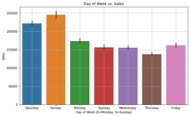
plt.show()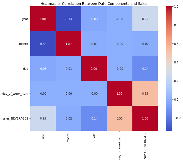
    

The code above shows a strong correlation between the sales and days of the week and between the sales and the years. Let's draw the corresponding graphs to verify the variations.

Data Visualization

Day of the Week vs. Sales

        Python
       
plt.figure(figsize=(10, 6))
sns.barplot(x='day_of_week', y='sales_BEVERAGES', data=dfc)
plt.title('Day of Week vs. Sales')
plt.xlabel('Day of Week (0=Monday, 6=Sunday)')
plt.ylabel('Sales')
plt.grid(True)
plt.show()

Year vs. Sales

    Python
   
 

   plt.figure(figsize=(10, 6))
sns.lineplot(x='year', y='sales_BEVERAGES', data=dfc, marker='o')
plt.title('Year vs. Sales')
plt.xlabel('Year')
plt.ylabel('Sales')
plt.grid(True)
plt.show()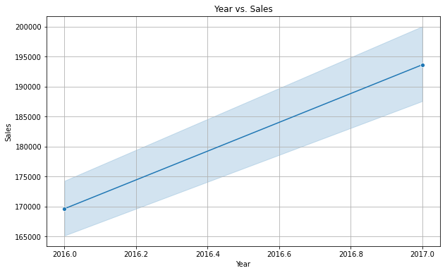
  

There is a clear indication that the sales are high on weekends and lesser on Thursdays. Also, yearly sales are increasing every year. It is a linear trend which means there are not many variations.

Month-Year vs. Sales

Let's quickly verify the variation with the year-month combination as well.

    Python
   
 

   dfc['month_year'] = dfc['date'].dt.to_period('M')
plt.figure(figsize=(16, 8))
sns.barplot(x='month_year', y='sales_BEVERAGES', data=dfc)
plt.title('Month vs. Sales')
plt.xlabel('Month-Year')
plt.ylabel('Sales')
plt.grid(True)
plt.show()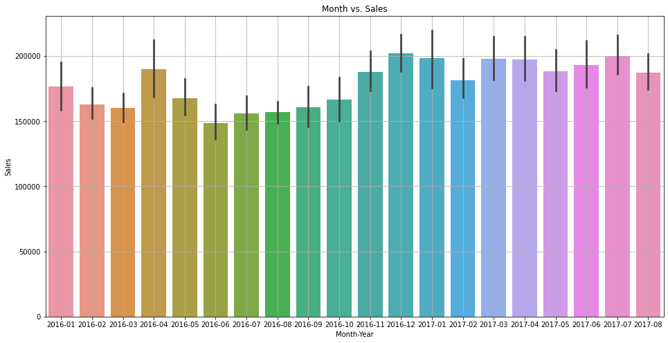
  

Due to limited data, it is not very clear, but it seems like sales are higher in the month of December and January.

Average Sales Calculation Per Year

    Python
   
 

   
#Evaluate the average sales of the year on monthly bais.
a = dfc[dfc['year'].isin([2016,2017])].groupby(["year", "month"]).sales_BEVERAGES.mean().reset_index()
plt.figure(figsize=(10, 6))
sns.lineplot(data=a, x='month', y='sales_BEVERAGES', hue='year', marker='o')

# Enhance the plot with titles and labels
plt.title('Average Sales for 2016 and 2017')
plt.xlabel('Month')
plt.ylabel('Average Sales')
plt.legend(title='Year')
plt.grid(True)

# Show the plot
plt.show()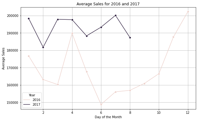
  

ACF vs PACF (Not Required for LSTM as Such)

This step is generally used with the ARIMA model, but still, it will give you some good visibility around the window size used later.

    Python
   
   fig, ax = plt.subplots(1,2,figsize=(15,5))
sm.graphics.tsa.plot_acf(dfc.sales_BEVERAGES, lags=365, ax=ax[0], title = "AUTOCORRELATION\n")
sm.graphics.tsa.plot_pacf(dfc.sales_BEVERAGES, lags=180, ax=ax[1], title = "PARTIAL AUTOCORRELATION\n")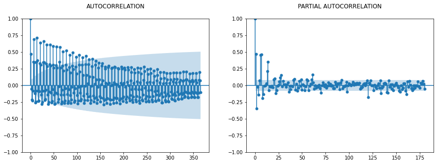

Take out the subset of the data for the trend analysis. Only fetch out the sales_BEVERAGAES, as we are going to perform a single variate analysis in this exercise:

    Python
   
   df1=dfc[["date",'sales_BEVERAGES']]
df1.head()

    
       date    sales_BEVERAGES

  2016-01-02  250510.0

  2016-01-03  299177.0

  2016-01-04  217525.0

  2016-01-05  187069.0

  2016-01-06  170360.0

This line plots the sales_BEVERAGES column from df1, starting from the second element (index 1) to the end. The exclusion of the first data point ([1:]) is used to avoid a specific outlier.

This would filter df1 to only include rows where sales_BEVERAGES is greater than 20,000. Again a step is required to take out the outliers.

    Python
   
   plt.plot(df1['sales_BEVERAGES'][1:])
df1=df1[df1['sales_BEVERAGES']>20000]
df2=df1['sales_BEVERAGES'][1:]
df2.shape

(589,)

MinMaxScaler

MinMaxScaler is from the sklearn.preprocessing library to scale the data in the df2 series. This is a preprocessing step in data analysis and machine learning tasks, especially when working with neural networks, as it helps to normalize the data within a specified range, typically [0, 1].

X scaled = X max −X min /X−X min

It is used here to improve the convergence process. Many machine learning algorithms that use gradient descent as an optimization technique (e.g., linear regression, logistic regression, neural networks) converge faster when features are scaled. If one feature’s range is orders of magnitude larger than others, it can dominate the objective function and make the model unable to learn effectively from other features.

    Python
   
   scaler=MinMaxScaler()
scaler.fit(df2.values.reshape(-1, 1))# Convert the PeriodIndex to DateTimeIndex if necessary
df2=scaler.transform(df2.values.reshape(-1, 1))

    Python
   
   plt.plot(df2)

I have not used the function below, but still, I have included it with a short explanation. I used the time-series generator instead of it, though both of them will perform the same task. You can use any of them. The function is designed to convert a Pandas DataFrame into input-output pairs (X, y) for use in machine learning models, particularly those involving time series data, such as LSTMs.

window_size: An integer indicating the number of time steps in each input sequence, defaulted to 5
df_as_np converts the Pandas DataFrame to NumPy array to facilitate numerical operations and slicing.
Two lists will be created: X for storing input sequences and y for storing corresponding labels (output).

It iterates over the NumPy array, starting from the first index up to the length of the array minus the window_size. This ensures that each input sequence and its corresponding output value can be captured without going out of bounds. For each iteration, it extracts a sequence of length window_size from the array and appends it to X. This sequence serves as one input sample. The output value (label) corresponding to each input sequence is the next value immediately following the sequence in the DataFrame. This value is appended to y.

Example:

X=[1,2,3,4,5], y=6

X=[2,3,4,5,6], y=7

X=[3,4,5,6,7], y=8

X=[4,5,6,7,8], y=9

and so on...

    Python
   
 

   def df_to_X_y(df, window_size=5):
  df_as_np = df.to_numpy()
  X = []
  y = []
  for i in range(len(df_as_np)-window_size):
    row = [[a] for a in df_as_np[i:i+window_size]]
    X.append(row)
    label = df_as_np[i+window_size]
    y.append(label)
  return np.array(X), np.array(y)
  

    Python
   
   WINDOW_SIZE = 5
X1, y1 = df_to_X_y(df2, WINDOW_SIZE)
X1.shape, y1.shape
print(y1)

    
  

   [143636. 152225. 227854. 263121. 157869. 136315. 132266. 120609. 141955.
 220308. 251345. 158492. 136240. 143371. 115821. 135214. 204449. 231483.
 141976. 128256. 129324. 113870. 137022. 209541. 245481. 182638. 154284.
 149974. 134005. 167256. 207438. 152830. 133559. 157846. 154782. 132974.
 144742. 190061. 219933. 166667. 150444. 142628. 124212. 146081. 203285.
 234842. 153189. 134845. 137272. 120695. 137555. 208705. 229672. 158195.
 179419. 170183. 135577. 152201. 227024. 245308. 155266. 132163. 137198.
 119723. 141062. 201038. 223273. 144170. 135828. 147195. 121907. 143712.
 202664. 216151. 148126. 130755. 148247. 149854. 149515. 182196. 195375.
 143196. 130183. 129972. 129134. 178237. 247315. 280881. 168081. 146023.
 145034. 122792. 149302. 209669. 236767. 146607. 134193. 138348. 115020.
 136320. 186935. 308788. 303298. 301533. 249845. 213186. 191154. 233084.
 238503. 148627. 135431. 136526. 114193. 146007. 232805. 282785. 181088.
 161856. 154805. 135208. 155813. 233769. 193033. 167064. 142775. 146886.
 125988. 138176. 206787. 247562. 159437. 135697. 133039. 120632. 140732.
 198856. 235966. 146066. 118786. 119655. 118074. 173865. 169401. 210425.
 154183. 189942. 144778. 136640. 136752. 200698. 237485. 143265. 122148.
 123561. 103888. 120510. 177120. 209344. 145511. 122071. 130428. 117386.
 138623. 201641. 188682. 156605. 144562. 130519. 110900. 127196. 186097.
 211047. 143453. 120127. 120697. 111342. 163624. 221451. 240162. 171926.
 141837. 141899. 117203. 137729. 186086. 205290. 148417. 127538. 120720.
 108521. 139563. 191821. 206438. 148214. 123942. 128434. 115017. 129281.
 178923. 188675. 148783. 124377. 132795. 107270. 133460. 191957. 216431.
 180546. 152668. 145874. 128160. 148293. 193330. 206605. 157126. 137263.
 138205. 135983. 164500. 166578. 180725. 158646. 147799. 147254. 127986.
 150082. 187625. 211220. 155457. 142435. 141334. 124207. 134789. 176165.
 197233. 147156. 133625. 145155. 147069. 181079. 238510. 261398. 183848.
 164550. 154897. 123746. 138299. 206418. 235684. 145080. 122882. 121120.
 116264. 143598. 200090. 235321. 141236. 132262. 129414. 110130. 136138.
 192610. 221098. 143488. 122181. 123595. 112182. 142867. 251375. 279121.
 172823. 146150. 146410. 120057. 143269. 202566. 247109. 153350. 125318.
 129236. 111697. 138234. 197333. 258559. 151406. 129897. 127212. 124603.
 144526. 192343. 241561. 142098. 124323. 128716. 120153. 136370. 194747.
 232250. 148589. 182070. 215033. 180293. 193535. 208685. 270422. 187162.
 166081. 164618. 129184. 150597. 222661. 291398. 165265. 160177. 181322.
 138887. 167311. 220970. 278158. 172392. 151843. 157465. 133102. 170648.
 223057. 263835. 177635. 140124. 164748. 178953. 185360. 255126. 297968.
 182323. 207703. 178510. 140546. 163758. 209125. 260947. 168443. 148518.
 159319. 146315. 169151. 226210. 270298. 196844. 194254. 198153. 198308.
 226894. 236331. 227027. 177554. 192477. 186177. 240693. 243518.   4008.
 335235. 243422. 211239. 175975. 189393. 261820. 297197. 186203. 171274.
 164531. 145461. 174206. 252034. 301353. 199820. 184129. 176227. 144535.
 162192. 264633. 299512. 191891. 167718. 160219. 125294. 156006. 226837.
 257357. 155191. 165171. 192241. 155016. 173306. 256450. 265030. 171537.
 156490. 161764. 132978. 164050. 220696. 255490. 169350. 129329. 147599.
 137081. 156814. 246049. 213733. 167601. 157364. 148629. 149845. 182391.
 230937. 168924. 165020. 212594. 204522. 180400. 186437. 257990. 276118.
 169456. 157163. 150271. 147502. 177393. 245596. 288397. 178705. 163684.
 173812. 164418. 188890. 259101. 297490. 192579. 172289. 167424. 153886.
 182043. 257097. 284616. 188293. 164975. 177997. 136349. 188660. 336063.
 264738. 188774. 184424. 181898. 153189. 171158. 228604. 262298. 170621.
 163715. 171716. 177420. 179465. 216599. 233163. 175805. 158029. 149701.
 144429. 169675. 236707. 285611. 175184. 161949. 164587. 143934. 180469.
 250534. 249008. 303807. 200529. 188754. 149629. 161279. 233814. 287104.
 166843. 145619. 147196. 135028. 154026. 244193. 206986. 179114. 169098.
 165675. 133381. 161718. 227900. 280849. 169143. 151437. 153706. 136779.
 212870. 212127. 254132. 171962. 158403. 174304. 166771. 204402. 278488.
 339352. 214773. 184706. 181931. 152212. 178063. 242234. 311184. 176821.
 158624. 158633. 142765. 181072. 250214. 245520. 179095. 173553. 154251.
 125467. 160086. 218486. 263497. 166889. 140339. 143776. 136268. 170346.
 271027. 297619. 199766. 173857. 170074. 150965. 178964. 232222. 262375.
 179826. 162466. 158262. 149968. 181719. 246513. 283097. 193199. 170182.
 163361. 163747. 183117. 229380. 245466. 188077. 160403. 156176. 141686.
 191922. 249085. 274030. 195504. 215546. 204566. 156806. 187818. 225481.
 250784. 179419. 160636. 153010. 156449. 189111. 182318. 202354. 174832.
 170773.]
  

TimeSeriesGenerator

The TimeseriesGenerator utility from the Keras library in TensorFlow is a powerful tool for generating batches of temporal data. This utility is particularly useful when working with sequence prediction problems involving time series data. This aims to simplify the creation of a TimeseriesGenerator instance for a given dataset.

Params

data: The dataset used to generate the input sequences
targets: The dataset containing the targets (or labels) for each input sequence; In many time series forecasting tasks, the targets are the same as the data because you are trying to predict the next value in the same series.
length: The number of time steps in each input sequence (specified by n_input).
batch_size: The number of sequences to return per batch (set to 1 here, which means the generator yields one input-target pair per batch)

Advantages

Using a TimeseriesGenerator offers several advantages:

Memory efficiency: It generates data batches on the fly and hence, is more memory-efficient than pre-generating and storing all possible sequences.
Ease of use: It integrates seamlessly with Keras models, especially when using model training routines like fit_generator.
Flexibility: It can handle varying lengths of input sequences and can easily adapt to different forecasting horizons.

    Python
   
   def ts_generator(dataset,n_input):
    generator=TSG(dataset,dataset,length=n_input,batch_size=1)
    return generator

    Python
   
 

   #Number of steps to use for predicting the next step
WINDOW_SIZE = 30
#This defines the number of features, in our case it is one and it should be sames as the count of neurons in the Dense Layer
n_features=1
generator=ts_generator(df2,WINDOW_SIZE)
  

The code snippet provided iterates over a TimeseriesGenerator object, collecting and aggregating all batches into two large NumPy arrays: X_val for inputs and y_val for targets.

    Python
   
 

   X_val,y_val=generator[0]
for i in range(len(generator)):
    X2, Y2 = generator[i]
    print("X:", X2)
    #print("Y:", type(Y))
    X_val = np.vstack((X_val, X2))
    y_val = np.vstack((y_val, Y2))
X_val=X_val[1:]
y_val=y_val[1:]
X_val=X_val.reshape(X_val.shape[0],WINDOW_SIZE,n_features)
y_val=y_val.flatten()
print(X_val.shape)
print(y_val)
  

Split this dataset into training, validation, and testing sets based on percentages of the dataset's total length.

    Python
   
 

   #l_percent is set to 85%, marking the cutoff for the training set.
#h_percent is set to 90%, marking the end of the validation set and the beginning of the test set.
l_percent=0.85
h_percent=0.90
#l_cnt is the index at 85% of df2, used to separate the training set from the validation set.
#h_cnt is the index at 90% of df2, used to separate the validation set from the testing set.
l_cnt=round(l_percent * len(df2))
h_cnt=round(h_percent * len(df2))
#Splits for dataset creation
val_sales,val_target=X_val[l_cnt:h_cnt],y_val[l_cnt:h_cnt]
train_sales,train_target=X_val[:l_cnt],y_val[:l_cnt]
test_sales,test_traget=X_val[h_cnt:],y_val[h_cnt:]

print(val_sales.shape,val_target.shape,train_sales.shape,train_target.shape,test_sales.shape,test_traget.shape)

  

(30, 30, 1) (30,) (502, 30, 1) (502,) (29, 30, 1) (29,)

Setting up a Deep Learning Model Using Keras (TensorFlow Backend) for a Time Series Forecasting Task

The code below sets up a deep learning model using Keras (TensorFlow backend) for a time series forecasting task, integrating callbacks for better training management and defining an LSTM-based neural network.

Callback Setup

EarlyStopping: Stops training when a monitored metric has stopped improving after a specified number of epochs (patience=50); This helps in avoiding overfitting and saves computational resources.
ReduceLROnPlateau: Reduces the learning rate when a metric has stopped improving, which can lead to finer tuning of models. It decreases the learning rate by a factor of 0.25 after the performance plateaus for 25 epochs, with the minimum learning rate set to 1e-9 (0.000000001).
ModelCheckpoint: It saves the model after every epoch but only if it's the best so far (in terms of the loss on the validation set). It saves only the weights to a directory named model/, which helps in both saving space and potentially avoiding issues when model architecture changes but the training script does not.

Layer Setup

Layer1: The first LSTM layer has 128 units and returns sequences. This means it will return the full sequence to the next layer rather than just the output of the last timestep. This setup is often used when stacking LSTM layers. It uses ReLU activation and includes dropout and recurrent dropout of 0.2 to combat overfitting.
Layer2: The second LSTM layer has 64 units and does not return sequences, indicating it's the final LSTM layer and only returns output from the last timestep. Similar to the first LSTM, it uses ReLU activation with dropout and recurrent dropout settings.
Layer3: A dense layer with 64 units acts as a fully connected neural network layer following the LSTM layers to interpret the features extracted from the sequences.
Layer4: The final dense layer with a single unit is typical for regression tasks in time series, where you predict a single continuous value.

Normally, the ReLU function is used with LSTM layers, but I have seen better results with tanh in the prelim analysis so I included this.

    Python
   
 

   from tensorflow.keras.callbacks import EarlyStopping, ModelCheckpoint, ReduceLROnPlateau
callbacks = [
EarlyStopping(patience=20, verbose=1),
ReduceLROnPlateau(factor=0.25, patience=10, min_lr=0.000000001, verbose=1),
ModelCheckpoint('model/', verbose=1, save_best_only=True,  save_weights_only=True)
]
model=Sequential()
model.add(LSTM(128,activation='tanh',dropout=0.2, recurrent_dropout=0.2,return_sequences=True,input_shape=(WINDOW_SIZE,n_features)))
model.add(LSTM(64, activation= 'tanh', dropout=0.2, recurrent_dropout=0.2))
model.add(Dense(64))

model.add(Dense(n_features))
model.summary()
  

Model: "sequential_6"
_________________________________________________________________
 Layer (type)                Output Shape              Param #   
=================================================================
 lstm_16 (LSTM)              (None, 30, 128)           66560     
                                                                 
 lstm_17 (LSTM)              (None, 64)                49408     
                                                                 
 dense_15 (Dense)            (None, 64)                4160      
                                                                 
 dense_16 (Dense)            (None, 1)                 65        
                                                                 
=================================================================
Total params: 120193 (469.50 KB)
Trainable params: 120193 (469.50 KB)
Non-trainable params: 0 (0.00 Byte)
_________________________________________________________________

Compile a Keras model with specific settings for the optimizer, loss function, and evaluation metrics.

Optimizer

optimizers.Adam(lr=.000001): This specifies the Adam optimizer with a learning rate (lr) of 0.000001. Adam is an adaptive learning rate optimization algorithm that has become the default optimizer for many types of neural networks because it combines the best properties of the AdaGrad and RMSProp algorithms to handle sparse gradients on noisy problems.
Learning rate: Setting the learning rate to a very small value, like 0.000001, makes the model training take smaller steps to update weights, which can lead to very slow convergence. This low value is used when you need to fine-tune a model or when training a model where larger steps might cause the training process to overshoot the minima.

Loss Function

loss='mse': This sets the loss function to Mean Squared Error (MSE), which is commonly used for regression tasks. MSE computes the average squared difference between the estimated values and the actual value, making it sensitive to outliers as it squares the errors.

    Python
   
   # Compile the model

#cp1 = ModelCheckpoint('model/', save_best_only=True)

model.compile(optimizer=optimizers.Adam(lr=.000001), loss= 'mse', metrics = ['mean_squared_error'])

It specifies how the training should be conducted, including the datasets to be used, the number of training epochs, and any callbacks that should be applied during the training process.

epochs=200: The number of times the model will work through the entire training dataset

    Python
   
   model.fit(train_sales, train_target, validation_data=(val_sales, val_target) ,epochs=200, callbacks=callbacks)

Epoch 1/200
16/16 [==============================] - 1s 72ms/step - loss: 0.0055 - mean_squared_error: 0.0055 - val_loss: 0.0110 - val_mean_squared_error: 0.0110
Epoch 2/200
16/16 [==============================] - 2s 98ms/step - loss: 0.0063 - mean_squared_error: 0.0063 - val_loss: 0.0067 - val_mean_squared_error: 0.0067
Epoch 3/200
16/16 [==============================] - 1s 71ms/step - loss: 0.0062 - mean_squared_error: 0.0062 - val_loss: 0.0119 - val_mean_squared_error: 0.0119
Epoch 4/200
16/16 [==============================] - 1s 71ms/step - loss: 0.0058 - mean_squared_error: 0.0058 - val_loss: 0.0097 - val_mean_squared_error: 0.0097

training_loss_per_epoch: This retrieves the training loss for each epoch from the model's history object. The training loss is a measure of how well the model fits the training data, decreasing over time as the model learns.
validation_loss_per_epoch: Similarly, this retrieves the validation loss for each epoch. Validation loss measures how well the model performs on a new, unseen dataset (validation dataset), which helps to monitor for overfitting.
Overfitting: If your training loss continues to decrease, but your validation loss begins to increase, this may indicate that the model is overfitting to the training data.
Underfitting: If both training and validation losses remain high, this might suggest that the model is underfitting and not learning adequately from the training data.
Early stopping: By examining these curves, you can also make decisions about using early stopping to halt training at the optimal point before the model overfits.

    Python
   
   training_loss_per_epoch=model.history.history['loss']
validation_loss_per_epoch=model.history.history['val_loss']
plt.plot(range(len(training_loss_per_epoch)),training_loss_per_epoch)
plt.plot(range(len(validation_loss_per_epoch)),validation_loss_per_epoch)

load_model is a function from Keras that allows you to load a complete model saved in TensorFlow's Keras format. This includes not only the model's architecture but also its learned weights and its training configuration (loss, optimizer).

    Python
   
   from tensorflow.keras.models import load_model
model1=load_model('model/')

Fetching out the dates from the original DataFrame to set it in the predictions for visibility. Since we are using the window size of 30, the first output/target/prediction will be generated after window_size. Accordingly, manipulate the dates for all three datasets.

The below code is designed to extract specific date ranges from a DataFrame to align them with corresponding training, validation, and test datasets. This is particularly useful when you want to track or analyze results over time or relate them to specific events or changes reflected by dates.

    Python
   
 

   date_df=df1[df1['sales_BEVERAGES']>20000]
date_df.count()
####Fetching the dates from the df1 for the train dataset
train_date=date_df['date'][WINDOW_SIZE - 1:l_cnt +  WINDOW_SIZE - 1]
print(train_date.count())
####Fetching the dates from the df1 for the val dataset
val_date=date_df['date'][l_cnt +  WINDOW_SIZE - 1:h_cnt +  WINDOW_SIZE - 1:]
print(val_date.count())
u_date=h_cnt + 1 + WINDOW_SIZE -1
test_date=df1['date'][h_cnt +  WINDOW_SIZE - 1: ]
test_date.count()
  

502
30

Training Data Actual Value vs Predicted Value

    Python
   
 

   #This function is used to generate predictions from your pre-trained model on the train_sales dataset.
train_predictions = model1.predict(train_sales).flatten()
# Applies the inverse transformation to the scaled predictions to bring them back to their original scale.
train_pred=scaler.inverse_transform(train_predictions.reshape(-1, 1))
t=scaler.inverse_transform(train_target.reshape(-1, 1))
#print(train_pred.shape)
#Creating a dataframe with Actual and predictions
train_results = pd.DataFrame(data={'Train Predictions':train_pred.flatten(), 'Actuals':t.flatten(),'dt':train_date })
train_results.tail(20)
  

16/16 [==============================] - 0s 14ms/step
(502, 1)

	Train Predictions	Actuals	dt
512	195323.593750	171962.000000	2017-05-29
513	164753.343750	158403.000000	2017-05-30
514	155985.328125	174304.000000	2017-05-31
515	153953.828125	166771.000000	2017-06-01
516	184015.109375	204402.000000	2017-06-02
517	246616.375000	278488.000000	2017-06-03
518	251735.953125	339352.000000	2017-06-04
519	187089.109375	214773.000000	2017-06-05
520	169009.390625	184706.000000	2017-06-06
521	160138.390625	181931.000000	2017-06-07
522	158093.562500	152212.000000	2017-06-08
523	186708.203125	178063.015625	2017-06-09
524	254521.234375	242234.000000	2017-06-10
525	263513.468750	311184.000000	2017-06-11
526	191338.093750	176820.984375	2017-06-12
527	168676.562500	158624.000000	2017-06-13
528	158633.203125	158633.000000	2017-06-14
529	153251.765625	142765.000000	2017-06-15
530	180730.171875	181071.984375	2017-06-16
531	251409.359375	250214.000000	2017-06-17

Below is a graphical representation of actual and predicted values of the training data for the first 100 pointers:

    Python
   
 

   plt.plot(train_results['dt'][:100],train_results['Train Predictions'][:100],label='pred')
plt.plot(train_results['dt'][:100],train_results['Actuals'][:100],label='Actual')
plt.legend()
plt.xticks(rotation=45)
plt.plot(figsize=(18,10))
plt.show()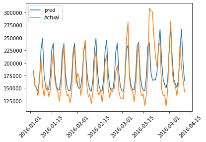
  

Validation Data Actual Value vs Predicted Value

    Python
   
 

   ##This function is used to generate predictions from your pre-trained model on the validation dataset.
val_predictions = model1.predict(val_sales).flatten()
# Applies the inverse transformation to the scaled predictions to bring them back to their original scale.
val_pred=scaler.inverse_transform(val_predictions.reshape(-1, 1))
v=scaler.inverse_transform(val_target.reshape(-1, 1))
print(val_pred.shape)
#Creating a dataframe with Actual and predictions
val_results = pd.DataFrame(data={'Val Predictions':val_pred.flatten(), 'Actuals':v.flatten(),'dt':val_date })
val_results.head()
  

1/1 [==============================] - 0s 62ms/step
(30, 1)

	Val Predictions	Actuals	dt
532	265612.906250	245519.984375	2017-06-18
533	186157.468750	179094.984375	2017-06-19
534	167559.578125	173553.000000	2017-06-20
535	158167.000000	154251.000000	2017-06-21
536	155162.000000	125467.000000	2017-06-22

Below is a graphical representation of actual and predicted values of the validation data:

     Python
    
 

    plt.plot(val_results['dt'],val_results['Val Predictions'],label='pred')
plt.plot(val_results['dt'],val_results['Actuals'],label='Actual')
plt.legend()
plt.xticks(rotation=45)
plt.plot(figsize=(18,10))
plt.show()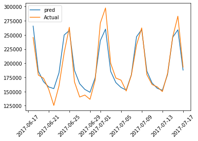
   

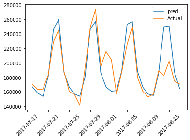
Test Data Actual Value vs Predicted Value

     Python
    
 

    #This function is used to generate predictions from your pre-trained model on the test dataset.
test_predictions = model1.predict(test_sales).flatten()
# Applies the inverse transformation to the scaled predictions to bring them back to their original scale.
test_pred=scaler.inverse_transform(test_predictions.reshape(-1, 1))
te=scaler.inverse_transform(test_traget.reshape(-1, 1))
print(test_pred.shape)
#Creating a dataframe with Actual and predictions
test_results = pd.DataFrame(data={'Test Predictions':test_pred.flatten(), 'Actuals':te.flatten(),'dt':test_date })
test_results.head()
   

1/1 [==============================] - 0s 35ms/step
(29, 1)

	Test Predictions	Actuals	dt
562	166612.140625	170182.000000	2017-07-18
563	158095.812500	163361.000000	2017-07-19
564	153619.515625	163747.000000	2017-07-20
565	181217.421875	183117.015625	2017-07-21
566	246784.828125	229380.000000	2017-07-22

      Python
     
     plt.plot(test_results['dt'],test_results['Test Predictions'],label='pred')
plt.plot(test_results['dt'],test_results['Actuals'],label='Actual')
plt.legend()
plt.xticks(rotation=45)
plt.plot(figsize=(18,10))
plt.show()

Machine learning Time series Data (computing) Neural Networks (journal) Python (language)

Opinions expressed by DZone contributors are their own.

Related

Trending