Ensuring Predictable Performance in Distributed Systems
In this article, we'll explore the concept of tail percentiles and how to assess and manage randomness in them.
Join the DZone community and get the full member experience.
Join For FreeLatency spikes can be a frustrating reality for many organizations, especially regarding tail percentiles. It's not uncommon to see unexplained spikes in latency, especially when there's no deliberate focus on predictability.
Consider a scenario where a web service must render a personalized web page. To provide a good user experience, ensuring low latency for 90% to 95% of requests is necessary. However, the page's content may require dozens or even hundreds of sub-requests from various components, each with its own variance and randomness. While each component may have low latency in 99% of cases, it might not be enough to guarantee consistent end-user latency. This highlights the importance of having the right Service Layer Objectives (SLOs) for each component to ensure overall system performance.
Reducing variance requires understanding statistics and probabilities, which can be challenging for even trained statisticians. However, simple mental models and heuristics can help to develop intuition and better understand system mechanics. This can be achieved by running mathematical simulations and playing with parameters to see how each dimension affects the end result.
What exactly is randomness? Philosophically, there's no strict definition for it. It's a matter of perspective, and both "everything is random" and "nothing is" can be defensible. In practical terms, randomness is defined as an outcome that cannot be predicted in advance. However, if there's a long-term pattern or distribution of outcomes, it can be considered random for practical purposes.
In this blog post, we'll explore the concept of tail percentiles and how to assess and manage randomness in them. Interactive Codelabs will be provided in some sections to help deepen your understanding of the concepts.
Mathematical Modeling
The first step in reducing tail latency is to create a model that accurately represents the characteristics of your system. Keep the model as simple as possible while ensuring it still captures the essential elements of your system. Simplicity makes it easier to understand and reduces the risk of misinterpretation. But beware of oversimplifying, as it could result in an inadequate representation of the system. The goal is to strike a balance between simplicity and accuracy.
Working with models helps train your brain to assign appropriate weight to various inputs. This exercise helps improve your professional intuition and engineering skills and saves time by quickly eliminating incorrect assumptions and avoiding costly dead-end solutions.
We can deconstruct the latency of operation into two major components:
latency = fixed_price + random_delay
fixed_price— the fixed cost represents the minimum cost of performing work, such as CPU cycles for computations or time for data to travel, which cannot be reduced.random_delay— the unpredictable surplus caused by various factors such as thread contention, packet loss, or network congestion.
Having a set of micro-benchmarks that cover all major components of the system can help determine the fixed cost. By collecting enough samples, the fixed cost can be calculated as the lower boundary, while the random delay can be derived from the observed variance. This can be measured as the standard deviation and latency percentiles (also see Measuring network service performance).
Intuitive Understanding of Percentiles
Percentile metrics such as p50, p90, p99, p99.9, etc., are commonly used to measure request latency. Simply put, percentiles indicate the base cost of hitting "bad" conditions. For example, p90 represents the worst 10% of causes, and p99 represents the worst 1% of causes.
Imagine a service that has a cache L1 with an 80% hit rate. This means that in 20% of cases, data has to be read from the database. The p80 latency would represent the minimum cost of falling back to the database. If the database also has a cache L2 with a 50% hit rate, the latency percentiles would look like this:
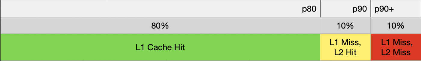
p80— latency when theL1cache has data.p90— whenL1doesn't have data butL2has data.p90+— when the DB has to read data from the disk.
Higher percentiles indicate worse luck and can result from various causes such as failure handling, lost packets, resource saturation, retries, rollbacks, etc.
Randomness Budget
Percentiles can also be viewed in terms of a randomness budget. For instance, if we want to guarantee a p95 at a certain level, we have a 5% randomness budget that can be used for cache misses, fallbacks, etc. The challenge then becomes how to divide this budget between upstream dependencies.
Note that probability is not additive, so arithmetic division cannot be used for calculations. The split depends on how upstream dependencies are called, whether in parallel or serially. The method of calculation would vary for different call patterns.
Percentiles of Multiple Operations
Let's begin by establishing our terminology:
- Service — a component that generates the end result.
- Dependency — an upstream component that is called by the Service to get data.
- Operation — a unit of work done by Service.
- Sub-request — a unit of work done by Dependency. We assume all sub-requests within an operation are independent.
What is the relationship between the operation latency and the sub-request latency? Let's take a look at two cases:
- Multiple sub-requests are performed in parallel.
- Multiple sub-requests are performed sequentially.
Parallel Sub-Requests and Tail Percentiles
Let's say a service needs to make multiple sub-requests to Dependency in parallel:
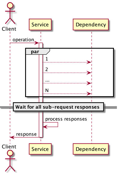
Assuming that we're interested in the p99 of operation latency, would it be just the sub-request that falls under the p99 category? Actually, no. Let's examine why that is. The simplest case is when there are two requests.
As you remember from above, p99 — means the worst 1%. So what is the probability that both requests will happily fall into the 99% of good cases?
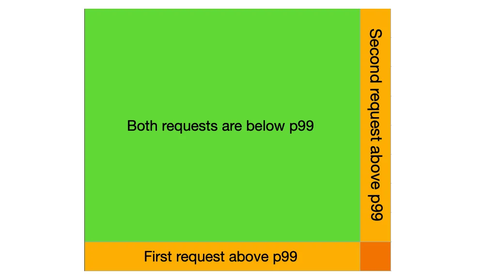 A geometrical illustration of the probability of independent events.
The probability of two independent events occurring together is calculated by multiplying their individual probabilities. For example, if each event has a probability of 0.99 (or 99%), the combined probability of both events happening is 0.99 * 0.99 = 0.9801.
It's important to convert percentages to values between 0 and 1 when working with probabilities. This allows us to perform mathematical operations with them.
As a result, the chance of not reaching the 99th percentile for a sub-request is 0.9801, or 98.01%. This means that the worst 1% of sub-requests will occur in 2% of service operations.
Let's do the same math in the case of 10 sub-requests:

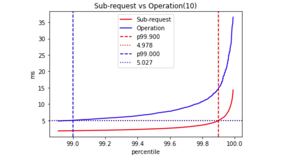
Now, the worst 1% of sub-requests will affect 9.5% of our operations. This highlights the issue of relying solely on the p99 of a dependency. The question is, what is the appropriate percentile to examine for sub-request latency? It involves finding the reverse - if we want the green square's area to be 0.99, then its side length corresponds to the p99.5 of Dependency latency. In the case of 10 sub-requests, the corresponding percentile is p99.9 of Dependency latency.
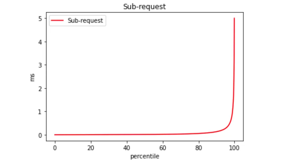
Here is how the percentile point function (PPF) may look in the case of 10 sub-requests:
You can play around with an empirical demonstration of this formula to get a better sense by trying out different parameters using this Codelab.
Sequential Rub-Request Execution
Now let's change our scenario. Suppose we need the outcome of one sub-request to proceed with the next one. In this case, the sub-requests have to be executed in sequence:
To make it simple, let's assume all services have a similar latency pattern that is generally consistent but shows some deviation in its outliers.
Typically, a log-normal distribution is effective in modeling network latency.
A log-normal process is the statistical realization of the multiplicative product of many independent random variables, each of which is positive.
Examples of log-normal distributed values in the real world (besides an operation's latency):
- The length of comments posted in Internet discussion forums follows a log-normal distribution.
- Users' dwell time on online articles (jokes, news, etc.) follows a log-normal distribution.
- The length of chess games tends to follow a log-normal distribution.
- Rubik's Cube solves, both general or by person, appear to follow a log-normal distribution.
This approach can also be used for Pareto distribution, which may be better suited for systems with heavy tail variances. You can experiment with this by switching the distribution to Pareto in the Codelabs and observing the impact on results. The same mathematical calculations can still be used even if the variance mostly affects the tail.
For example, if the PPF looks like this:
To get the variance, we can subtract the minimum (i.e. fixed_price) value from the latency. Then we can calculate operation latency by adding the fixed_price and variance:
latency(n) = n * fixed_price + variance(n)
The heuristic approach may not be entirely accurate in certain cases, but it's effective for small numbers of sub-requests, up to several dozen. For example, if two requests are executed in parallel, the sub-request percentile would be p99.5, while it would be p99.53 in the case of sequential execution:
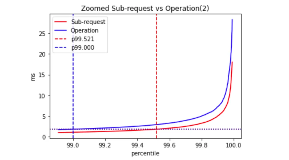
Why does this heuristic work? Because outliers have a significant impact on the tail, and the likelihood of two outliers occurring together is very low, we can ignore it.
Let's try the model with ten sub-requests:
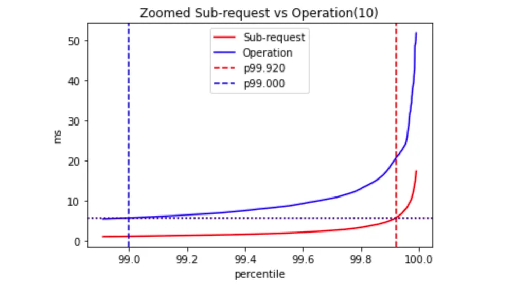
The actual percentile of the single sub-request latency is p99.92.
If we use this heuristic, then estimated_p99(operation)=5.97mswhile the actual_p99(operation)=6.62ms. I.e., the difference is ~10%.
However, if we apply a naive estimation, i.e. naive_p99(operation)=10*p99(sub_request), we'll get 11.81ms. This estimation is overly pessimistic and is ~80% away from the actual value.
Please note this is a simple heuristic applicable under certain conditions. For existing systems, you may need to simulate this using factual measurements and distributions.
Conclusion
In real-life situations, different components have different latency distributions. It is crucial to focus on the most impactful ones, which are usually the dependencies with the largest variance or the highest number of incoming requests. The more a dependency is called, the greater its impact on end-user latency. Therefore, it is essential to set appropriate Service Layer Objectives for low-level components that may be stricter than those for high-level components (e.g., p99.9, p99.95, or even p99.99).
Although building predictable services on top of unpredictable dependencies may be challenging, it is possible in some cases. For example, improving the tail with request hedging can help mitigate the impact of components with high variance.
Published at DZone with permission of Eugene Retunsky. See the original article here.
Opinions expressed by DZone contributors are their own.
Comments