Monte Carlo Simulations at Scale: Stock Price Prediction
Learn how to use AWS Batch to run Monte Carlo simulations efficiently and at scale, with a practical example from the financial sector (stock price prediction).
Join the DZone community and get the full member experience.
Join For FreeMonte Carlo methods are a class of methods based on the idea of sampling to study mathematical problems for which analytical solutions may be unavailable. The basic idea is to create samples through repeated simulations that can be used to derive approximations about a quantity we’re interested in, and its probability distribution.
In this post, we’ll describe how you can use AWS Batch to run Monte Carlo simulations optimally and efficiently at scale. We’ll illustrate using an example from the financial sector: the stock price prediction problem.
Some Background to the Monte Carlo Method
The Monte Carlo method was developed as a statistical computing tool in the mid-1940s near the advent of computing machines. John von Neumann and Stanislaw Ulam first came up with the idea of using random numbers generated by a computer in order to solve problems encountered in the development of the atomic bomb. The title of their paper, “The Monte Carlo method," which gave birth to the Monte Carlo method, is a reference to the famous casino in Monaco. You can read their paper yourself in the Journal of the American Statistical Association, 44:335–341, 1949.
Monte Carlo methods are widely used in a variety of fields like finance, physics, chemistry, and biology (and more). In these fields, many realistic models of systems of interest usually involve the assumption that at least some of the underlying variables behave in a random way. For example, in the financial domain, the prices of different assets (like stocks) are assumed to evolve in time by following a random (or stochastic) process. The Monte Carlo simulation method uses random sampling to study the properties of such systems by simulating on a computer the stochastic behavior of these systems. In detail, a computer is used to randomly generate values for the stochastic variables that influence the behavior of the system. Then for each stochastic simulation, samples of the quantities of interest are computed, which are further analyzed by methods of statistical inference.
The Monte Carlo method can also be used for problems that have no inherent probabilistic structure, like computing high-dimensional multivariate integrals or solving huge systems of linear equations. While the main advantages of Monte Carlo methods over other techniques are ease of implementation and parallelization, it does have some drawbacks. One of the main drawbacks of Monte Carlo simulations is their slower rate of convergence compared to some other specialized techniques, like so-called quasi-Monte Carlo methods. When you have a large number of variables bound to distinct constraints, this method might be computationally challenging. It can be demanding in terms of computing power and computing time to approximate a solution.
In this post, we’ll use Monte Carlo methods to value and analyze some financial assets by simulating the various sources of uncertainty affecting their value (usually done with the help of stochastic asset models), and then determine the distribution of their value over the range of resultant outcomes. We’ll walk through technical details to efficiently scale and optimize your Monte Carlo simulations, but we won’t focus on any specific data preparation or processing steps.
Architecture Diagram
The architecture we will create is depicted in Figure 1.
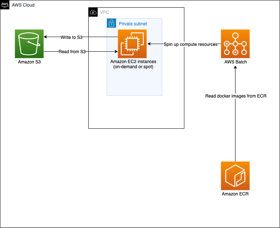
Figure 1: In this architecture, we’ll use Amazon S3 for data storage, AWS Batch for scheduling, ECR to source containers, and Spot Instances for large-scale and low-cost capacity.
In our architecture, we use several services:
- Amazon S3 to store input and output files: Amazon S3 is an object storage service that offers industry-leading scalability, data availability, security, and performance.
- Amazon ECR is used to store packaged Docker images. Amazon ECR is a fully managed container registry offering high-performance hosting, so you can reliably deploy application images and artifacts anywhere.
- AWS Batch array jobs are used to process datasets that are stored in Amazon S3 and presented to Amazon EC2 compute instances. Batch is a fully managed service that helps you to run batch computing workloads at any scale.
Solution Overview
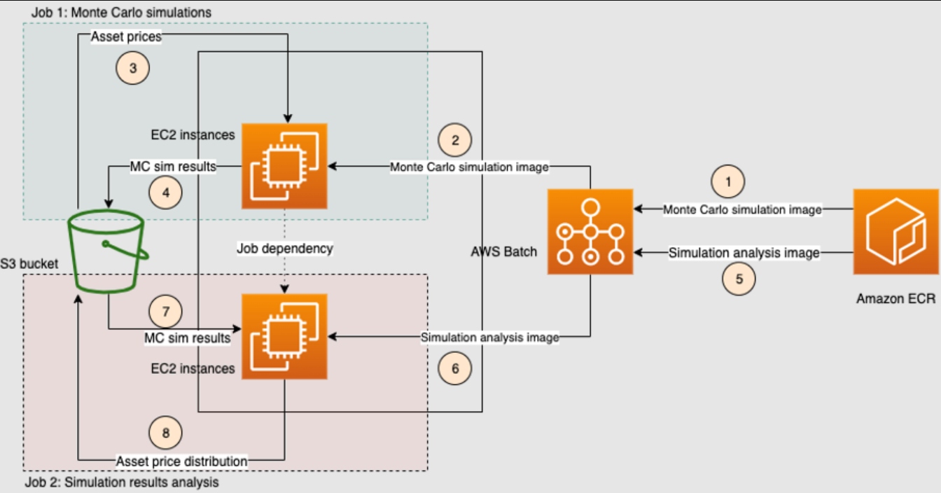
Figure 2: In our solution, the key services that enable large-scale elasticity are AWS Batch and Amazon S3.
The Monte Carlo simulations workflow proceeds in the form of two serial jobs:
- In Job 1, we use the array jobs feature of Batch to submit multiple jobs in parallel, each of which runs Monte Carlo simulations. The final results of this step are stored as CSV files in an Amazon S3 bucket. The detailed steps involved in Job 1 are as follows:
- AWS Batch retrieves the Docker image for performing Monte Carlo simulations from Amazon ECR.
- AWS Batch spins up a cluster of Amazon EC2 instances (On-Demand or Spot) to run the Docker image from step (1) in the diagram.
- Each AWS Batch job from the array retrieves the input data from an S3 bucket and performs a Monte Carlo simulation.
- Each AWS Batch job stores the results of its own Monte Carlo simulation in the same S3 bucket as step (4).
- In Job 2, we submit another AWS Batch job, that will be run only after the successful completion of the first array job using the job dependencies feature of AWS Batch. This job takes as input the results of the Monte Carlo simulations of the first step and performs custom post-processing and analysis. The results of this analysis are also stored in the original S3 bucket. The detailed steps involved in Job 2 are as follows:
- In step (5), AWS Batch retrieves the Docker image for performing analysis on the Monte Carlo results of Job 1 from Amazon ECR.
- In step (6), AWS Batch spins up a single EC2 instance for running the Docker image from step (5).
- In step (7), the Batch job from step (6) retrieves the results of the Monte Carlo simulations of Job 1 from the S3 bucket of Job 1.
- In step (8), the Batch job stores the result of the analysis in the same S3 bucket as step (7).
To get a sense of the scaling of this solution, in the use-case where Job 1 is a job array consisting of 5 jobs, the maximum runtime across all the array jobs was around 2 seconds, and Job 2 for analyzing the results of the Monte Carlo simulations of the first job also completed in 2 seconds.
This solution can be trivially scaled up to 10,000 simulations (the maximum size for array jobs supported in AWS Batch currently) by submitting Job 1 with the size field in the array-properties parameter set to the desired number of simulations. Because all the other services we use in this solution (like Amazon S3 and Amazon ECR) are inherently scalable, too, there’s no additional work involved to get there.
To apply this to the stock price prediction problem, we use sample data obtained from yfinance, which is a reliable, threaded, and Pythonic way to download historical market data from Yahoo! finance.
In finance, quantities like stock prices are usually assumed to evolve in time following a stochastic path. For example, in the standard Black–Scholes model, the stock price is assumed to evolve in time by a stochastic process known as “Geometric Brownian Motion” (GBM). Many problems in mathematical finance involve the computation of a particular integral (like finding the arbitrage-free value of a particular derivative). In some cases, these integrals can be computed analytically, but more often they’re computed using numerical integration or by solving a partial differential equation (PDE).
However, when the number of dimensions (or degrees of freedom) in the problem is large, PDEs and numerical integrals become intractable, and in these cases, Monte Carlo methods often give better results. In particular, for more than three or four state variables, formulae such as Black–Scholes (i.e., analytic solutions) just don’t exist, while other numerical methods (like the Binomial options pricing model and finite difference methods) face several difficulties, making them impractical. In these cases, Monte Carlo methods converge to the solution more quickly than numerical methods, need less memory, and are easier to program. Monte Carlo methods can also deal with derivatives that have path-dependent payoffs in a fairly straightforward manner.
Advantages of This Approach
There are a lot of advantages of this architectural design, compared to traditional approaches for performing Monte Carlo simulations.
First, since AWS Batch is a managed service there’s no need to install and manage batch computing software or server clusters to run your jobs. Batch also dynamically provisions the right quantity and type of compute resources (like CPU or memory-optimized instances) based on the volume and specific resource requirements of the jobs in the queue. And we have more to say on this topic in our documentation on allocation strategies. This is a significant freedom, compared to the constraints of fixed-capacity clusters.
With a bring-your-own container approach, you can choose any framework and algorithm without extensive changes to your code base.
And finally, just using Amazon EC2 Spot Instances can save you up to 70% on your compute costs.
Next Steps
In this post, we’ve described how to efficiently scale and optimize your Monte Carlo simulations using AWS Batch. We also discussed the technical details of the architecture, and hopefully, you’ll see some of the advantages of using this approach. An almost identical setup can be used for other use cases, like option pricing or portfolio analysis.
You can get started implementing the solutions described here by following the directions in the aws-samples GitHub repo. We’d love to hear how this helps.
Published at DZone with permission of Sai Sharanya Nalla. See the original article here.
Opinions expressed by DZone contributors are their own.
Comments